
Paperis Articles
Inequality and Social Stratification — This Month's Allowance, the Piggy Bank Handed Down
What does a line like 'the top 10% hold 44% of the wealth' actually measure? Income and wealth, the different rulers for inequality, and the research on how far those gaps carry over to the next generation.
Your field's papers, as audio
Pick your fields and journals — Paperis summarizes the key papers and turns them into audio. Listen on your commute.
Start Paperis free →Inequality and Social Stratification — This Month's Allowance, the Piggy Bank Handed Down
The Sentence "The Top 10% Own 44%"
This kind of sentence frequently appears in stories about wealth: "The top 10% of households with the most wealth hold 44% of the total wealth of all households." This is a figure presented as a starting point by a study that built an economic model tailored to Korean data (DOI: 10.22841/kerdoi.2026.42.3.004). It means that the households at the top—about one out of every ten houses in descending order of wealth—together hold close to half of all household wealth.
When you hear this number, questions follow. Is this a lot? Does earned money differ by this much as well? Does that difference pass straight down to children? This article covers the terms and rulers needed to read those questions. The examples are mainly drawn from Korea, and the concepts apply to any society.
As a guide, we use a single classroom. Ten classmates each have this month's allowance, and at home, piggy banks they have been filling for several years. If you follow along while comparing allowances and piggy banks, it becomes easy to read past the headlines and understand what the numbers actually measure. However, actual statistics measure by household rather than individual students, and adult earnings differ from a set allowance. The classroom is used only to help visualize the shape of the numbers.
This Month's Allowance, and a Piggy Bank Full of Years
Let us say there are two friends who receive the same allowance. One friend's piggy bank was given a lump sum by a relative, while the other friend's piggy bank had no such thing. Even if this month's allowance is the same, the weight of their piggy banks is vastly different.
An adult's household finances are also viewed through these two tracks. Income is the money that comes in over a fixed period, commonly a year. Wages earned from work and dividends generated from owned assets are examples of income (OpenStax Introduction Sociology 3e 9.1). Household income in South Korea is broken down into the share earned through work, the share earned through business, and the share generated from assets such as interest and rent (DOI: 10.18207/criso.2020..127.60).
Wealth is the sum of all money and property owned at a given point in time, minus debts. Money in bank accounts, houses, and land all fall into this category (OpenStax Introduction Sociology 3e 9.1). In news and research, the amount before subtracting debt is sometimes called assets, and the amount after is called net worth. If allowance is income, the piggy bank is wealth.
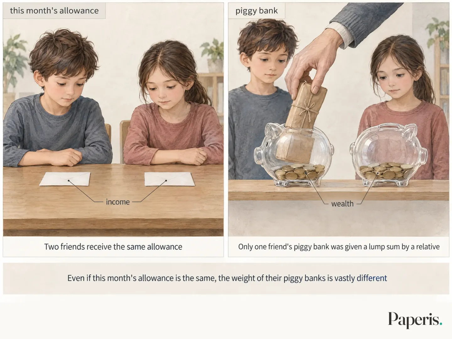
Statistics usually count both of these on a household basis (DOI: 10.18207/criso.2020..127.60). A household is a unit of people living together and sharing a livelihood in one home; if you live alone, you are a household of one.
The difference on the piggy bank side can be enormous. Using 2021 data in the United States, the top 1% holding the most wealth owned one-third of the nation's total wealth, while the bottom half combined owned 2% (OpenStax Introduction Sociology 3e 9.2). In a South Korean study that divided elderly people and those soon to be elderly into three groups based on when they were born, wealth inequality was clearly greater than income inequality across all three groups (DOI: 10.17000/kspr.27.3.202009.45).
Why do differences in the piggy bank last so long? Allowance is received and spent anew each month, but the piggy bank remains and can be passed down to the next generation. A sociology textbook covering American society explains that as wealth passes to children, the structure of social classes is carried over into the next generation (OpenStax Introduction Sociology 3e 9.2).
Wealth differences in South Korean households are mainly divided by real estate. In data from the early 2000s, the share that real estate contributed to wealth inequality was roughly 6 to 7 times that of financial assets (KCI ART001357023). During periods when housing prices rose, the gap between households that owned homes and those that did not was the main driver of increased wealth inequality (DOI: 10.46228/KJE.31.1.3). A study comparing South Korea with the United States and Spain starts by positioning South Korea as a country with a lower level of wealth inequality than the United States, but with a higher share of real estate. In that analysis, the wedge between the group that owned homes and the group that did not accounted for a share of total wealth inequality that was clearly larger than in the other two countries (KCI ART002239560).
Income and wealth do not always move in the same direction. There is an analysis showing that in South Korea during the 2000s, the two grew together. This is different from the pattern in several developed nations, where when one side was uneven, the other tended to be relatively even (KCI ART001727819). In the first half of the 2010s, both decreased, and over the few years that followed, income inequality decreased while wealth inequality increased again (DOI: 10.18207/criso.2020..127.60).
The magnitude of income inequality and wealth inequality differs, and they sometimes move in the same direction and sometimes in opposite directions.
If You Line Ten People Up
Now let us line ten people up in a single file, from the friend with the least allowance to the friend with the most. There are a few different rulers that summarize the line at a glance.
The most widely used ruler is the Gini coefficient (DOI: 10.1002/9781405165518.wbeosg045.pub2). The Gini coefficient is a number measuring inequality between 0 and 1, where 0 is absolute equality and 1 is maximum inequality where one person has everything. If all ten people receive exactly 10,000 won each, it is 0; the more one person takes all the allowance while the other nine get not a single penny, the closer it gets to the 1 end. There is also the Gini index, which is multiplied by 100 (DOI: 10.1002/9781405165518.wbeosg045.pub2). The Gini coefficient measuring Korean household wealth was 0.61 in the study from the first section (DOI: 10.22841/kerdoi.2026.42.3.004), and 0.660 in another study measured using 2006 data (KCI ART001357023). Because these two values use different data and measurement points, they cannot be strung together to conclude that inequality has decreased.
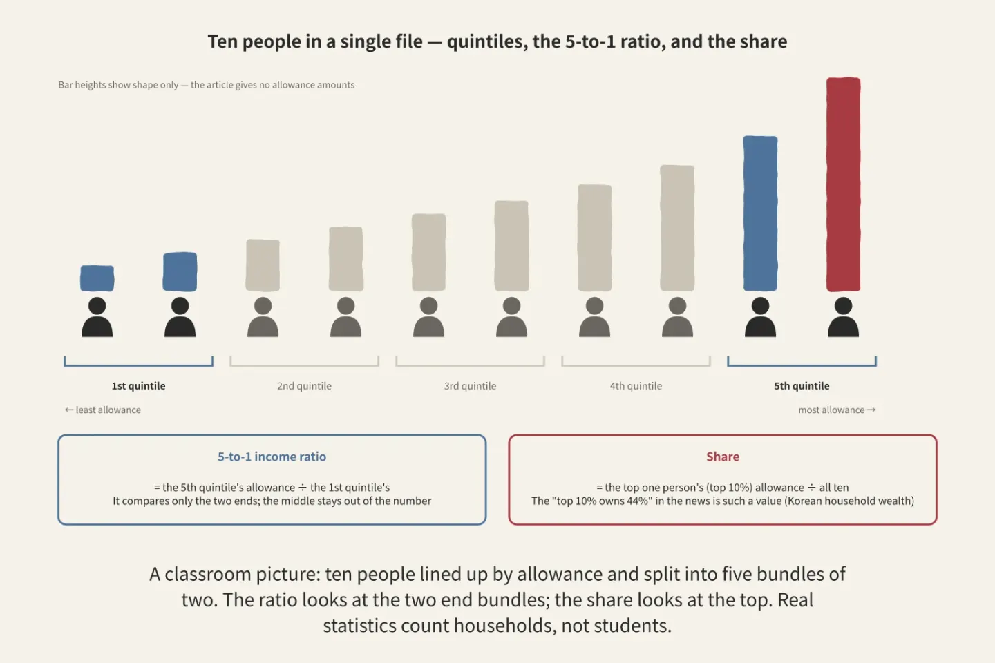
Figure: a diagram Paperis drew using only what the article says
There are also rulers that chop the line into pieces. Income quintiles/deciles are groups created by lining up all households in order of income and dividing them into equal-sized bundles. When divided into five, the 1st quintile is the group earning the least and the 5th quintile is the group earning the most; when divided into ten, it goes up to the 10th decile. In a classroom, that would be five bundles of two people each.
The 5-to-1 income ratio represents how many times larger the income of the top 5th quintile group is compared to the bottom 1st quintile group. Along with the Gini coefficient, it is considered a core indicator of income distribution in Korea (KCI ART003284008). In Korea, the 5-to-1 ratio remained large for several years following the foreign exchange crisis, and one study views this change as relying significantly on structural factors alongside the ups and downs of the business cycle (KCI ART001114520). Ratios comparing the top 10% and bottom 10% are also used. However, because such ratios compare only both ends, the circumstances of the people in the middle of the line do not enter the numbers (OpenStax Introduction Sociology 3e 10.1).
The share is a value representing what percentage of total income or wealth a certain group accounts for. The "top 10% owns 44%" from the first section is a share.
Ratios look at both ends, shares look at the very top, and the Gini coefficient looks at the entire line. Therefore, relying on just a single ruler causes things to be missed. One study points out that the Gini coefficient has a property where measured inequality can actually shrink even when the incomes of people at the very top increase, and concludes that because of this, the recent increase in income inequality in the United States appears smaller than it actually is when viewed through the Gini coefficient (DOI: 10.1111/roiw.12638).
The rulers that measure inequality are not singular, and each ruler looks at a different place in the line.
Two Ways of Thinking About Poverty
The word "poor" overlaps two thoughts. They are the questions of how low an income must be to count as poor, and what that line is drawn against. Depending on where that line is drawn, the ways of measuring poverty split into an absolute side and a relative side (DOI: 10.1093/actrade/9780198716471.003.0003).
The relative side starts from the middle of the line. Median income is the income of the household standing right in the middle when all households are lined up in order of income. In a classroom, it is right between the fifth and sixth friends. Even if a single large allowance at the very end of the line pulls up the average, it cannot move the middle spot.
Relative poverty is a plight where, even if one secures what is strictly necessary to eat and sleep, one cannot live as ordinarily as the average person in that society. That line is commonly drawn relative to median income. A Korean study also defined relative-poverty households based on the median value of household income adjusted for the number of household members (DOI: 10.35175/KRS.2019.20.1.5). A sociology textbook covering the United States gives half of the median income as an example of that line (OpenStax Introduction Sociology 3e 9.2). Poverty lacking even basics like meals or a place to stay is counted separately from this (OpenStax Introduction Sociology 3e 10.2).
The line of relative poverty moves along with society. If everyone's income doubles equally, the middle income also doubles, and the proportion of people below the line stays the same. Therefore, even if a country grows wealthy, relative poverty may not decrease.
What is subtracted from income before looking at it also changes the number. In a study measured using two years of data from the Korean Labor and Income Panel Study, when measured again using the income left after subtracting housing costs like rent, both poverty and income inequality rose (DOI: 10.33900/KAPS.2021.32.2.9).
Because relative poverty is a line drawn relative to the middle of society, it does not decrease on its own even when society grows wealthy.
Same Ruler, Different Data
Even the same Gini coefficient varies depending on what data was used and how it was adjusted and measured. Household surveys do not capture very high incomes well. Therefore, in a study that recalculated the Gini coefficient for 1998–2015 by supplementing the top with national tax statistics, the corrected values were roughly 10–18% larger than the original values (DOI: 10.20464/kdea.2017.23.3.1). Since 2010, the original Gini coefficient has declined slightly, whereas the corrected Gini coefficient tended to rise (DOI: 10.20464/kdea.2017.23.3.1).
The two surveys also diverge. In a study comparing South Korea's two representative surveys, the Household Financial Welfare Survey and the Korea Labor and Income Panel Study, the Gini coefficient rose in one and fell in the other after 2021 (DOI: 10.17298/kky.2025.31.2.003). The discrepancy arose mainly because people reported their incomes differently in the two surveys (DOI: 10.17298/kky.2025.31.2.003).
Inequality figures can only be read when both the ruler and the data are disclosed.
Social Class, and Moving Between Spots
The line in the classroom was formed based on this month's allowance alone. Society's line has multiple criteria. Social stratification is the structure in which people are divided and positioned up and down according to criteria such as wealth, income, education level, occupation, and family background. What sociology asks in this structure is not why a particular person stood at the front, but rather why people with similar family backgrounds or living situations cluster on certain sides of the line (OpenStax Introduction Sociology 3e 9.1).
Social class is a group of people who share a similar position in society because their conditions, such as income, wealth, education level, family background, and occupation, are alike.
How rigid a class structure is lies somewhere between two extreme pictures. One extreme is a society where positions are determined solely by effort and ability, but sociology textbooks view such a society as an ideal that has existed only in theory, never in reality. The other extreme is a caste system where it is nearly impossible to change one's birth position for a lifetime. Today's class-divided society lies between the two, meaning that while paths are open to move into different education levels and occupations from one's parents, one remains influenced by family and society (OpenStax Introduction Sociology 3e 9.1).
Regarding why social stratification exists, there is a long-standing explanation and criticism of it. In 1945, sociologists Kingsley Davis and Wilbert Moore argued that the more important a job is to society, the greater its rewards must be. In 1953, sociologist Melvin Tumin criticized this explanation for failing to explain educational inequality or inequalities based on race and gender, arguing instead that stratification actually prevents capable people from challenging for those positions (OpenStax Introduction Sociology 3e 9.4).
Social mobility is the movement of individuals or groups from one position to another within the social stratification system. Intergenerational mobility is when parents and their children occupy different social classes. In terms of the classroom, intergenerational mobility means that the spot where the parents stood and the spot where the child stands are different, and that spot could be higher up or lower down (OpenStax Introduction Sociology 3e 9.2).
Classrooms Where the Number of Seats Changes
The classroom analogy hits its limit here. While classroom seats are fixed in number each year, society changes the total number of seats itself. There was a time in the United States when nearly everyone moved up to higher seats together. This was during the first half of the 20th century, when the economy grew through industrialization (OpenStax Introduction Sociology 3e 9.2).
Therefore, mobility is counted in two ways. Absolute mobility simply counts how many people landed in a different class from their parents. Relative mobility strips away the share caused by changes in the total number of seats across society, looking instead at how similar the chances are for people of different origins to reach the same seats. If the number of big-piggy-bank seats grew so that most people ended up higher than their parents, absolute mobility is high; but if the order in line remains the same, relative mobility is low.
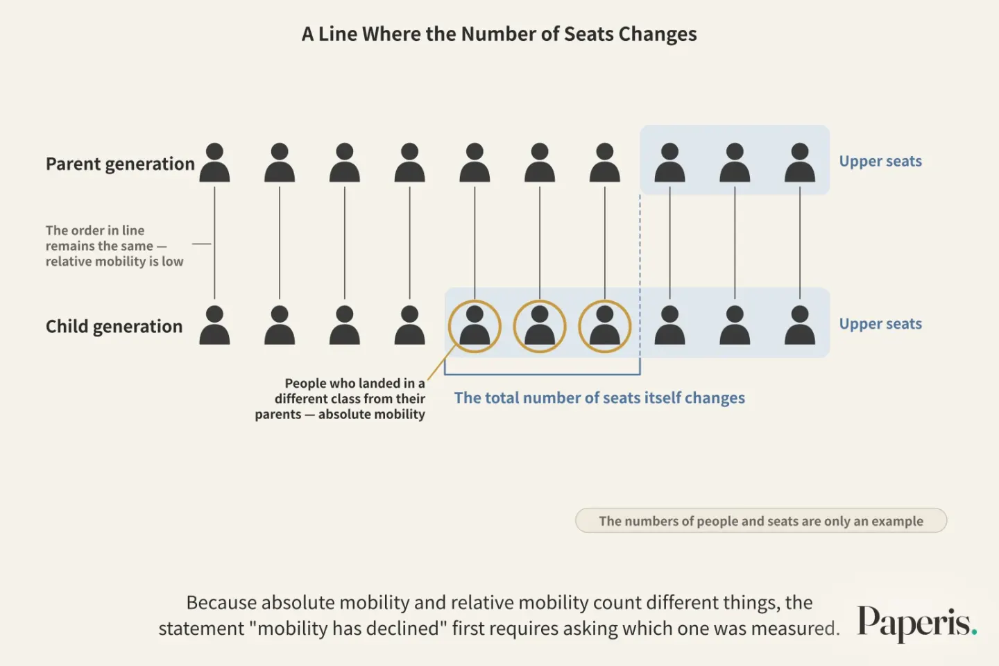
The two counts tell different stories. In the United States and seven European countries, people who moved upward during the 20th century increased up to those born around 1950, while those born afterward saw an increase in people moving downward. The biggest force driving upward movement was a massive shift in the composition of jobs during the 30 years after World War II. Education also made society more open as higher education expanded and the link between origins and educational attainment weakened (DOI: 10.11126/stanford/9781503610163.001.0001).
In South Korea, studies yield mixed results. In a study comparing two groups of men aged 30 to 49 in 1998 and 2018, absolute mobility remained relatively high, and relative mobility was statistically significantly higher in 2018 than in 1998. The proportion of people who moved upward decreased, which the authors view as a natural change driven by the shrinking proportion of parents who were farmers. The authors note that this result aligns with earlier studies concluding that intergenerational mobility in South Korea has not declined (DOI: 10.21562/kjs.2021.08.55.3.159). Another study comparing men born between the 1950s and 1980s in 10-year intervals suggested that relative mobility for those born in the 1970s and 1980s was lower than for the preceding generation. However, in the same study, the influence of parents' occupations on children's education and occupation was generally unclear and grew smaller for more recent generations, whereas the influence of children's own education on their occupation increased (DOI: 10.17000/kspr.32.2.202506.43). The authors interpret this as meaning that education has thus far served as a ladder for class mobility. They also point out that the wage premium for managerial and professional jobs has decreased, suggesting that class divisions may be more active in other domains—such as marriage or assets—than in occupation and income (DOI: 10.17000/kspr.32.2.202506.43).
The idea that "mobility has declined" is widely spread in South Korea through terms like the "spoon class theory." Noting that a gap exists between that perception and the measurement results, the aforementioned 2021 study writes that understanding that gap requires more sophisticated class distinctions, intergenerational income mobility studies, and research on those born after the 1990s to follow (DOI: 10.21562/kjs.2021.08.55.3.159).
Because absolute mobility and relative mobility count different things, the statement "mobility has declined" first requires asking which one was measured.
Parental Income and Children's Income
The inheritance of status is sometimes measured by income instead. Intergenerational income elasticity is a value showing how much of the income gap between parents carries over to the gap between children; it is 0 when there is no carryover at all, and closer to 1 means it carries over almost completely. A value of 0.3 means that, on average across many families, roughly 30 percent of the income gap between parents remains as a gap between children.
A study measuring this year by year using the Korean Labor and Income Panel Study data from 1998–2019 concludes that this value in South Korea has stayed around 0.27–0.30 since the late 2000s. In the same study, the unadjusted baseline estimate was 0.11–0.17, and it rose to 0.20–0.32 when reducing errors that occur when measuring children's income (DOI: 10.30885/RIE.2022.16.2.061). A working paper looking at sons born between 1958 and 1973 yielded around 0.4, and an earlier estimate using the same method was 0.22 (DOI: 10.2139/ssrn.2320329).
Whose income was measured and what kind of income it was affects why these numbers fluctuate. The former study measured household after-tax income (DOI: 10.30885/RIE.2022.16.2.061), while the working paper measured the earnings of sons and fathers (DOI: 10.2139/ssrn.2320329). Even so, the values from these studies lie somewhere between 0 and 1. Parents' income is linked to their children's income, but it does not transfer over as it is.
Inequality of Opportunity, Inequality of Outcome
Let us return to the classroom. If a child from a household with a heavier piggy bank can attend cram school more, the difference in allowance can lead to a difference in the starting line for the next year. There are two terms that divide this difference. Inequality of outcome is the degree to which what people actually earn and possess differs from person to person. Inequality of opportunity is when the prospects of what one will achieve in the future are split due to conditions one could not choose, such as parents' education level or where one was born.
In a study looking at the child and youth panel in South Korea from 2010 to 2016, private education spending by relative poverty households was roughly two-thirds of that of all households. Instead, the proportion that private education spending occupied in income was much higher for relative poverty households than for general households (DOI: 10.14816/sky.2019.30.1.155). The research team considers that such gaps can lead to problems that limit intergenerational mobility. This study did not measure mobility itself (DOI: 10.14816/sky.2019.30.1.155).
Which direction South Korea's inequality of opportunity moved in also varies by study. In a study that looked at incomes from 1990 to 2016 using father's education level as the starting condition, inequality of opportunity was low until the mid-1990s and grew rapidly through the foreign exchange crisis. However, looking only at household heads with a college degree or higher, it shrank significantly over the same period, and the authors view the educational gap of children according to the father's education level as a major pathway through which inequality of opportunity arises (DOI: 10.22841/kjes.2021.69.1.002). In another study that examined multiple starting conditions all at once using machine learning, South Korea's inequality of income opportunity was on a decreasing trend, but the influence of parental conditions such as parents' education and occupation was large, and the influence of the region where one was born and raised grew over time (KCI ART003057906).
When comparing countries, the two types of inequality showed a tendency to go together. In a study comparing nine developed countries in the 1990s, inequality of outcome and inequality of opportunity were strongly linked, the United States and Italy were the most unequal in both aspects, and Nordic countries had an income distribution according to background that was almost identical even before redistribution (DOI: 10.1111/j.1475-4991.2008.00289.x).
Inequality of outcome and inequality of opportunity ask different questions, but the two are connected to each other.
Does a More Uneven Society Move Less?
If you plot countries on a single chart, a striking pattern emerges. The Great Gatsby Curve is the relationship shown by plotting countries together, where countries with greater income inequality tend to have parents' and children's incomes resemble each other more. One review working paper summarizing this relationship gathered studies showing this curve across various contexts and outcomes (DOI: 10.2139/ssrn.4039480). The same paper shows that this relationship can arise mechanically simply from statistical models capturing how income moves, and organizes theories explaining it through people's behavior into five branches: family investment, technology, peer effects, politics, and aspirations.
However, a picture lining up countries at a single point in time does not tell us about changes over time. In the United States, inequality grew significantly, yet mobility did not decrease. A working paper looking at this puzzle using nearly a century of data from U.S. counties found that the relationship between changes in inequality and changes in mobility was weak and jagged over short intervals of about 20 years, but over long intervals of nearly 100 years, places where inequality grew more had a clear relationship where mobility decreased more (DOI: 10.2139/ssrn.7034829). The authors suggest that if high inequality persists, mobility could drop significantly in the long run even if it has not shrunk yet.
The picture can also flip depending on how you measure mobility. Another working paper reports that if you measure mobility not by the resemblance to parental income, but by how fast the incomes of people at the bottom rise, upward mobility actually turns out to be significantly higher in places with greater inequality (DOI: 10.2139/ssrn.5395430). The authors write that the two findings do not contradict each other, and that readers must first choose the ruler that fits the word "mobility."
While the tendency for inequality and the passing down of advantage to go together appears in various data, its causes and shape over time are still debated.
Reading Two Sentences of News
Let us read a sentence like this using what we have learned: "The Gini coefficient fell this year, reducing inequality."
First, we see whether it is income or wealth. The two inequalities have periods where they moved together and periods where they moved in opposite directions. Next, we see which survey it is. Since 2021, South Korea's two representative surveys showed Gini coefficients moving in opposite directions, and there were times when the Gini coefficient adjusted by supplementing top incomes moved in the opposite direction from the original value. Finally, we see whether other rulers point in the same direction. Since it has been pointed out that the Gini coefficient can actually fall when top incomes rise, we also check the top 10% share and the P90/P10 ratio. When all three point in the same direction, that sentence becomes sturdier.
Another is a sentence like this: "The ladder of social mobility is broken." Here, we first ask whether it is absolute mobility or relative mobility. Even if the number of people who moved upward decreases, it may be due to a change in the compositional structure of the parent generation's positions. Next, we ask whether it is class measured by occupation, elasticity measured by income, and who was looked at born in which year. The two Korean social mobility studies we looked at earlier looked only at men and gave different answers to the same question.
Neither sentence has the grounds to say it is wrong, nor the grounds to say it is right, within that single line. Numbers on inequality and mobility acquire meaning only when attached to what was measured, with which ruler, and using which data.
Where to Look Next
Why wealth takes on a shape that concentrates at the top, and the tail of that distribution, continue in "Why Wealth Concentrates — The Physics of Inequality". The story that the per-capita average of an entire country does not tell us about distribution is in "GDP and the Business Cycle — The Last Receipt, and the Day No Receipt Records", and how we measure jobs, the starting point of income, is in "Unemployment and Employment — Those in Line, Those Who Left It". "If People Who Take It Live Longer, How Were They Different to Begin With? — Confounding" covers why the mere fact that a parent's background and a child's income move together does not mean one caused the other.
How social structures and people's choices intertwine is covered in "What Is Society? — A Path Worn by Many Feet, and the Steps That Choose It". Aging continues in "Population — A House Divided into Floors by Age, and the People Who Move Up One Floor Each Year", the story of household shapes changing like single-person households in "Family — The Table We Share Every Night, and the Big Table We Set for the Holidays", and the burden of housing costs and regional disparities in "Cities and Regions — Gathered Around the Fire, Seats Beyond Its Light".
Source Papers
- "Introduction to Sociology 3e — 9.1 What Is Social Stratification?" (2021) — OpenStax Introduction Sociology 3e 9.1 — The distinction between wealth (the net value of money and property) and income (wages and dividends), the perspective that sociology focuses on which strata people of similar backgrounds gather in rather than individuals, the criteria for strata and class (including family background), closed systems (caste systems) and open systems (class, where individual choices and opportunities operate amidst the influence of family and society), and the view that pure meritocracy is merely an ideal and has never actually existed.
- "Introduction to Sociology 3e — 9.2 Social Stratification and Mobility in the United States" (2021) — OpenStax Introduction Sociology 3e 9.2 — How wealth passes down to children to maintain class structure in American class classification, the distribution of wealth in the United States (2021 data), upward and downward social mobility, intergenerational mobility, the structural upward mobility of almost everyone due to industrialization in the first half of the 20th century, and an example of the relative poverty line in American literary circles (half of median income).
- "Introduction to Sociology 3e — 9.4 Theoretical Perspectives on Social Stratification" (2021) — OpenStax Introduction Sociology 3e 9.4 — The Davis-Moore thesis (1945) and Tumin's critique of it (1953).
- "Introduction to Sociology 3e — 10.1 Global Stratification and Classification" (2021) — OpenStax Introduction Sociology 3e 10.1 — The income multiplier of the top 10% and bottom 10% (or 20%) is simple, but it is viewed by excluding the middle.
- "Introduction to Sociology 3e — 10.2 Global Wealth and Poverty" (2021) — OpenStax Introduction Sociology 3e 10.2 — The distinction between relative poverty (having necessities but falling short of society's average living standard) and extreme poverty (a lack of basic necessities such as food and safe housing).
- "Gini Coefficient" (2017) — DOI: 10.1002/9781405165518.wbeosg045.pub2 — The most widely used inequality measure, where 0 is complete equality and 1 is a state where one person holds everything, and the Gini index obtained by multiplying by 100.
- "Wealth Inequality in Korea: Limited Participation and Idiosyncratic Returns" (2026) — DOI: 10.22841/kerdoi.2026.42.3.004 — The top 10% share of Korean household wealth at 44% and a wealth Gini coefficient of 0.61, presented as starting facts by a model study tailored to Korean microdata (no data year in the abstract).
- "한국 사회 가구 소득과 자산의 불평등: 연구 성과와 과제" (2020) — DOI: 10.18207/criso.2020..127.60 — Long-term trends in household income and asset inequality (income inequality increased from the early 1990s to 2009 and decreased in the 2010s / asset inequality decreased in the first half of the 2010s and increased in the recent 3 years), and the distinction between labor, business, and asset income.
- "현재 노인과 미래 노인의 불평등 추이에 관한 연구: 코호트별 소득과 자산을 중심으로" (2020) — DOI: 10.17000/kspr.27.3.202009.45 — Asset inequality is significantly higher than income inequality across all three cohorts of current and prospective elderly.
- "한국 가계자산의 분배와 불평등 요인분해" (2009) — KCI ART001357023 — The 2006 net worth Gini of 0.660, where asset inequality is primarily determined by real estate distribution, with a contribution rate 6 to 7 times that of financial assets.
- "부동산 가격 변동과 경제불평등과의 관계 - 자산과 소득 불평등을 중심으로" (2024) — DOI: 10.46228/KJE.31.1.3 — The primary cause of worsening net worth inequality during periods of rising housing prices is the gap between home-owning households and non-homeowners.
- "국가 간 비교 관점에서 본 한국의 자산불평등- 한국, 미국, 스페인 주택자산의 불평등 효과를 중심으로 -" (2017) — KCI ART002239560 — Unlike the United States, Korea has a lower level of asset inequality and a higher proportion of real estate, and the contribution of inequality between home-owning and non-owning groups is significantly higher than in Spain and the United States.
- "한국에서 자산 및 소득의 이중적 불평등: 국제 비교 관점에서 본 한국의 불평등 구조의 특성" (2013) — KCI ART001727819 — While many developed countries show patterns where asset and income inequality offset each other, Korea has seen both rise together since the 2000s.
- "데이터 분석을 통한 지니계수와 소득분배 지표 기반 한국 소득불평등 구조 분석" (2025) — KCI ART003284008 — Examines the Gini coefficient, the 80/20 income quintile ratio, and the relative poverty rate as core income distribution indicators.
- "외환위기 이후 소득 5분위배율의 구조적 변화" (2005) — KCI ART001114520 — The 80/20 income ratio widened after the foreign exchange crisis and persisted for several years, likely driven significantly by structural factors as well as business cycle factors.
- "가구주 특성과 상대적 빈곤 :수도권과 비수도권의 비교" (2019) — DOI: 10.35175/KRS.2019.20.1.5 — Using Statistics Korea household income raw data, defining relative poverty households based on the median of equivalent total household income considering household size.
- "Inequality Measurement and The Rich: Why Inequality Increased More Than We Thought" (2023) — DOI: 10.1111/roiw.12638 — Concludes that the Gini coefficient has a property where income growth among the wealthy can reduce measured inequality, underestimating the recent increase in income inequality in the United States.
- "3. Measurement" (2018) — DOI: 10.1093/actrade/9780198716471.003.0003 — A book chapter. Setting the poverty line and the difference between absolute and relative poverty concepts.
- "상대적 빈곤층의 사교육비 지출규모와 변화추이" (2019) — DOI: 10.14816/sky.2019.30.1.155 — In the 2010–2016 panel, private education spending by the relative poverty group is about ⅔ of that of all households but constitutes a vastly higher proportion of income, which the authors judge could lead to the problem of limited intergenerational mobility (a premise within a policy proposal sentence; mobility itself is not measured).
- "주거비용이 빈곤 및 소득불평등에 미치는 영향 - 주거비를 감안한 빈곤 및 소득불평등의 측정 -" (2023) — DOI: 10.33900/KAPS.2021.32.2.9 — Poverty and income inequality increase after accounting for housing costs in the 17th and 24th waves of the Korea Labor and Income Panel Study.
- "보정 지니계수" (2017) — DOI: 10.20464/kdea.2017.23.3.1 — The Gini coefficient adjusted for the underreporting of high incomes in sample surveys using tax statistics (1998–2015) is 10% to 18% larger than the original value, with the original value declining slightly and the adjusted value increasing after 2010.
- "한국의 소득 불평등 추이: 서베이 데이터별 비교 분석" (2025) — DOI: 10.17298/kky.2025.31.2.003 — The Gini coefficients from the Household Finances and Living Conditions Survey and the Korea Labor and Income Panel Study diverge in opposite directions after 2021, with the difference mainly stemming from reporting behavior regarding income.
- "Education and Intergenerational Social Mobility in Europe and the United States" (2020) — DOI: 10.11126/stanford/9781503610163.001.0001 — A book. Upward mobility increased up to those born around 1950 in 7 US and European countries, followed by an increase in downward mobility; the main driver of upward mobility was occupational structure changes during the 30 years after World War II, and education also increased openness by expanding higher education and weakening the link between origin and education.
- "20년간의 세대 간 사회이동의 변화: 30~49세 두 남성 코호트 비교 분석" (2021) — DOI: 10.21562/kjs.2021.08.55.3.159 — Comparing 30–49-year-old men in 1998 and 2018. Absolute mobility rates remain high and the decline in upward mobility is a change driven by the decrease in farming parents, while relative mobility is significantly higher in 2018 — reaffirming the existing research conclusion that intergenerational mobility has not fallen, requiring subsequent research to understand the gap between perception and reality.
- "한국의 세대별 사회이동 변화:교육을 고려한 세대 간 직업 이동과 임금 분석" (2025) — DOI: 10.17000/kspr.32.2.202506.43 — Men born in the 1950s–1980s from the Korea Labor and Income Panel Study. While relative mobility appears to have declined for those born in the 1970s and 1980s, the influence of parental occupation is largely insignificant and smaller in more recent generations, whereas the impact of children's education has grown — the authors interpret that education has served as a ladder for class mobility thus far, suggesting that stratification may become active in other domains such as marriage and assets as the wage premium for managerial and professional jobs decreases.
- "한국의 세대 간 소득이동성의 연도별 추이 분석" (2022) — DOI: 10.30885/RIE.2022.16.2.061 — Korea Labor and Income Panel Study 1998–2019. Baseline estimates are 0.11–0.17, and when corrected for measurement error, 0.20–0.32, with the conclusion resting at the 0.27–0.30 level since the late 2000s.
- "Intergenerational Earnings Mobility in Korea" (2013) — DOI: 10.2139/ssrn.2320329 — A working paper. Intergenerational earnings elasticity for sons born between 1958 and 1973 is about 0.4 (compared to an earlier estimate of 0.22 using the same method).
- "한국노동패널과 가계동향조사를 이용한 소득기회불평등의 장기추세에 대한 연구" (2021) — DOI: 10.22841/kjes.2021.69.1.002 — Definition of inequality of opportunity; based on father's education level, income inequality of opportunity rose rapidly after the foreign exchange crisis from 1990 to 2016, dropped significantly among household heads with a college degree or higher, with educational gaps by father's education acting as the main pathway.
- "Inequality of Opportunity Analysis in Korea using Machine Learning" (2024) — KCI ART003057906 — When combining multiple environmental variables, income inequality of opportunity in Korea shows a declining trend, but the influence of parental background factors such as parents' education, industry, and occupation remains large, and the influence of birth and upbringing regions has increased.
- "INEQUALITY OF OPPORTUNITIES VS. INEQUALITY OF OUTCOMES: ARE WESTERN SOCIETIES ALL ALIKE?" (2008) — DOI: 10.1111/j.1475-4991.2008.00289.x — In 9 developed countries during the 1990s, there was a strong correlation between outcome inequality and opportunity inequality, with the US and Italy being the most unequal in both, while Nordic countries had nearly identical income distributions by origin even before redistribution.
- "The Great Gatsby Curve" (2022) — DOI: 10.2139/ssrn.4039480 — A working paper (review). Summarizes the positive relationship between cross-sectional income inequality and intergenerational income persistence, shows that this relationship can arise mechanically even from statistical models of income dynamics alone, and reviews five theoretical branches—family investment, technology, social influence, political economy, and aspirations—along with empirical studies from various contexts.
- "The Short and Long Run Dynamics of the Great Gatsby Curve" (2026) — DOI: 10.2139/ssrn.7034829 — A working paper. Using a century of data from US counties, the relationship between changes in inequality and changes in mobility is weak and unstable over 20-year intervals, but exhibits a significant negative relationship over spans approaching a century — concluding that if increases in inequality are not reversed, long-term mobility could be significantly reduced.
- "The Great Gatsby Curve: Upward Mobility, Persistence and Inequality" (2025) — DOI: 10.2139/ssrn.5395430 — A working paper (NBER). Upward mobility measured by the progressivity of income growth has a positive relationship with baseline inequality — suggesting this is merely a difference from persistence-based measurement and not a contradiction, and advising that the choice of measurement be aligned with the criterion.
Sources (27)
- Introduction to Sociology 3e — 9.1 What Is Social Stratification?
- Introduction to Sociology 3e — 9.2 Social Stratification and Mobility in the United States
- Introduction to Sociology 3e — 9.4 Theoretical Perspectives on Social Stratification
- Introduction to Sociology 3e — 10.1 Global Stratification and Classification
- Introduction to Sociology 3e — 10.2 Global Wealth and Poverty
- Gini CoefficientDOI 10.1002/9781405165518.wbeosg045.pub2
- Wealth Inequality in Korea: Limited Participation and Idiosyncratic ReturnsDOI 10.22841/kerdoi.2026.42.3.004
- 한국 사회 가구 소득과 자산의 불평등: 연구 성과와 과제DOI 10.18207/criso.2020..127.60
- 현재 노인과 미래 노인의 불평등 추이에 관한 연구: 코호트별 소득과 자산을 중심으로DOI 10.17000/kspr.27.3.202009.45
- 부동산 가격 변동과 경제불평등과의 관계 - 자산과 소득 불평등을 중심으로DOI 10.46228/kje.31.1.3
- 가구주 특성과 상대적 빈곤 :수도권과 비수도권의 비교DOI 10.35175/krs.2019.20.1.5
- Inequality Measurement and The Rich: Why Inequality Increased More Than We ThoughtDOI 10.1111/roiw.12638
- 3. MeasurementDOI 10.1093/actrade/9780198716471.003.0003
- 상대적 빈곤층의 사교육비 지출규모와 변화추이DOI 10.14816/sky.2019.30.1.155
- 주거비용이 빈곤 및 소득불평등에 미치는 영향 - 주거비를 감안한 빈곤 및 소득불평등의 측정DOI 10.33900/kaps.2021.32.2.9
- 보정 지니계수DOI 10.20464/kdea.2017.23.3.1
- 한국의 소득 불평등 추이: 서베이 데이터별 비교 분석DOI 10.17298/kky.2025.31.2.003
- Education and Intergenerational Social Mobility in Europe and the United StatesDOI 10.11126/stanford/9781503610163.001.0001
- 20년간의 세대 간 사회이동의 변화: 30~49세 두 남성 코호트 비교 분석DOI 10.21562/kjs.2021.08.55.3.159
- 한국의 세대별 사회이동 변화:교육을 고려한 세대 간 직업 이동과 임금 분석DOI 10.17000/kspr.32.2.202506.43
- 한국의 세대 간 소득이동성의 연도별 추이 분석DOI 10.30885/rie.2022.16.2.061
- Intergenerational Earnings Mobility in KoreaDOI 10.2139/ssrn.2320329
- 한국노동패널과 가계동향조사를 이용한 소득기회불평등의 장기추세에 대한 연구DOI 10.22841/kjes.2021.69.1.002
- INEQUALITY OF OPPORTUNITIES VS. INEQUALITY OF OUTCOMES: ARE WESTERN SOCIETIES ALL ALIKE?DOI 10.1111/j.1475-4991.2008.00289.x
- The Great Gatsby CurveDOI 10.2139/ssrn.4039480
- The Short and Long Run Dynamics of the Great Gatsby CurveDOI 10.2139/ssrn.7034829
- The Great Gatsby Curve: Upward Mobility, Persistence and InequalityDOI 10.2139/ssrn.5395430